Array formulas are powerful formulas in Excel that perform calculations using multiple ranges of cells. They are also known as CSE formulas because you must press CTRL + SHIFT + ENTER to tell Excel that you are inserting an array formula so that Excel can treat Range of cells as “ARRAYs”
Lets look at some of the basics. If we have a sound understanding of how Arrays work, we can understand how complex ARRAY formulas work and then we can write some creatively useful formulas on our own
An array is a collection of items (values, text etc) like {1,2,3,4,5}. If you type the formula =sum({{1,2,3,4,5}) in any cell you will get 15. If you type ={1,2,3,4,5}, Excel returns first element of the array
When two similar arrays are operated against another, the result is another array where every “nth” item of one array is operated against every “nth” item of other array
So
{1,2,3,4,5} + {6,7,8,9,10} returns {7,9,11,13,15}
{1,2,3,4,5} * {6,7,8,9,10} returns {6,14,24,36,50}
{10,2,3,4,50} > {6,7,8,9,10} returns {TRUE , FALSE , FALSE , FALSE , TRUE}
{“a”,”b”,”c”,”d”} = {“f”,”g”,”h”,”d”} returns {FALSE , FALSE , FALSE , TRUE}
{“a”,”b”,”c”,”d”} & {“f”,”g”,”h”,”d”} returns {“af”,”bg”,”bh”,”dd”}
Similarly When an array is operated against a value, each element of the array is operated against that Value resulting in a new array. So
{1,2,3,4,5} +1 returns {2,3,4,5, 6}
{1,2,3,4,5} >1 returns {FALSE , TRUE , TRUE , TRUE, TRUE}
If ({1,2,3,4,5} >1,{1,2,3,4,5},FALSE) returns {FALSE , 2 , 3 , 4, 5}
WITH THE ABOVE UNDERSTANDING LETS WORK ON ARRAY FORMULAS in EXCEL
Click here to Download the Illustrative Examples
1) PERFORMING INDEX MATCH WITH MULTIPLE CRITERION
In this simplified example, our challenge is to find the row (using formula of course) where all 3 criterion are met. i.e Name is Zubair, Country is Pakistan, Sex is Male.
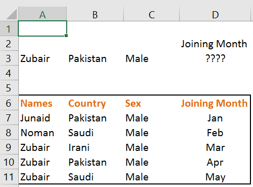
The Array Formula that will do the job is
=INDEX(D7:D11,MATCH(A3&B3&C3,A7:A11&B7:B11&C7:C11,0))
So how does it work. Recall from our understanding of arrays above that
A7:A11 & B7:B11 & C7:C11 should return {JunaidPakistanMale , NomanSaudiMale , ZubairIraniMale , ZubairPakistanMale , ZubairSaudiMale}
Therefore MATCH(A3&B3&C3,A7:A11&B7:B11&C7:C11,0) returns Match(ZubairPakistanMale,{JunaidPakistanMale , NomanSaudiMale , ZubairIraniMale , ZubairPakistanMale , ZubairSaudiMale},0)
so the answer is 4 (4th row of the data)
2) TESTING IF AN ITEM EXISTS IN A TABLE OR A LIST
Recall the “OR” function in Excel.
“OR” returns TRUE if at least 1 argument is TRUE
So OR (“A”=”A”,1=2) would return OR(TRUE,FALSE). The result is TRUE since one argument is TRUE
This Power of “OR” function can be used to check if an item exists in a range of cells
Example
OR (“Zubair”={“Hasan”, “Rayyan”, “John”,”Zubair”)) would return OR(False,False,False,True)
The result is TRUE since one argument is TRUE
Following is one way how I use it. The example is available in file you downloaded above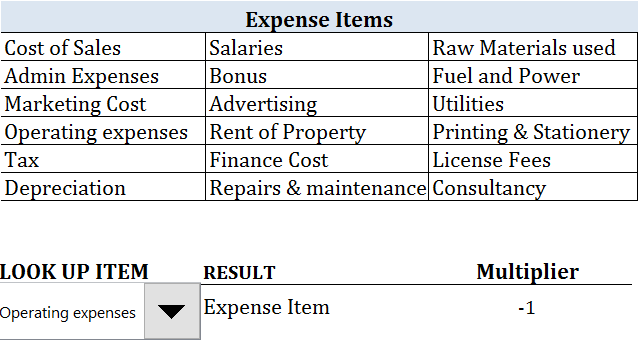
I use this Array Formula to check if an item I select from the DROP DOWN is an expense item. If an item is an EXPENSE item, it is multiplied by -1.
WHY? Because My company’s Information System stores expense items as “Negative” number which results in column charts hanging from the top.
So I use this Array Formula {=IF(OR(A17=Expenses),”Expense Item”,”Income Item”)} to “Check” if the user selection is an expense item and multiply it it with -1 so that chart shows positive numbers
Expenses is a named range. We can also use A3:C8
3) DETERMINE THE APPROPRIATE BAND OR GROUP BASED ON RANGE OF VALUES
Suppose HR uses following Parameters (Salary Ranges) to assign GRADES to Employees. Your objective is to determine the GRADE for the following six employees based on the parameter on the right
Try few formulas on your own before looking at the solution
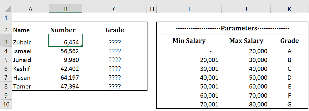
The required array formula is (For Cell C3)
{=INDEX($K$4:$K$10,MATCH(1,(B3>=$I$4:$I$10)*(B3<=$J$4:$J$10),0))}
This is how it works
B3>=$I$4:$I$10 returns {True,False,False,False,False}
B3<=$J$4:$J$10 returns {True,True,True,True,True}
In Excel “False” is equivalent to ZERO while “True” is equivalent to 1. You can test it by writing TRUE +1 or FALSE + 1 in any Cell in Excel
So (B3>=$I$4:$I$10)*(B3<=$J$4:$J$10) return {True,False,False,False,False}* {True,True,True,True,True}
{True,False,False,False,False}* {True,True,True,True,True} = {1,0,0,0,0}*(1,1,1,1,1}= {1,0,0,0,0}
So MATCH(1,(B3>=$I$4:$I$10)*(B3<=$J$4:$J$10),0) = MATCH(1,{1,0,0,0,0},0)= 1
So {=INDEX($K$4:$K$10, 1)} returns “A”
Please leave your feedback below.
If you have an interesting ARRAY formula to share please do share with me